Energy Conservation and Emission Reduction Strategies

~~~~~~~~~~~~~~

TDM Encyclopedia

Victoria Transport Policy Institute

~~~~~~~~~~~~~~~~~~~~

Updated 5 February 2021

---

This chapter examines the role that TDM can play in achieving air pollution emission reduction goals.

Introduction

Air pollution imposes many costs, including human health and environmental damages. As a result, many jurisdictions have emission reduction goals. Transportation Demand Management can play an important role in achieving these goals. Many TDM strategies can reduce emissions in addition to many other benefits; they are win-win solutions. Comprehensive analysis tends to justify TDM as part of emission reduction programs.

Although individually, most TDM strategies provide modest emission reductions, typically reducing just a few percent of total vehicle travel and pollution emissions, they generally become more effective if implemented as an integrated package that includes improvements to resource-efficient modes (walking, bicycling, ridesharing and public transit), plus incentives to choose the most efficient mode for each trip. For example:

� Residents of Transit Oriented neighborhoods typically drive less than half as much, and produce less than half the emissions, as residents of automobile-dependent urban fringe areas.

� Residents of Smart Growth regions typically drive 20-50% fewer annual miles than in sprawled regions.

� Commute Trip Reduction programs typically reduce affected commuters� vehicle travel by 5-15% if they rely only on information, and 10-30% if they also include Financial Incentives such as cost-recovery parking pricing or parking cash out.

� Efficient Parking Pricing typically reduces affected vehicle trips by 10-30% compared with unpriced parking.

� Comprehensive Walking and Cycling typically reduce automobile travel by 5-15%, and probably more in the future as e-scooters and e-bikes expand the range of trips that can be made by these modes.

� Pricing reforms, such as Fuel Tax Increases, Efficient Road Tolls, Pay-As-You-Drive Vehicle Insurance and other Distance Based Fees can reduce significant amounts of vehicle travel and emissions.

International and interregional comparisons indicate large variations in per capita vehicle travel and emissions, due largely to factors such as transportation and land use development policies, and fuel tax rates. For example, in 2018, U.S. residents averaged 16.6 tons of GHG emissions, 82% more than the 9.1 tons in Germany, and about twice as much as the 5.2 tons produced per capita in Britain. Similarly, in 2019 residents of Chicago, Portland and Seattle drove less than 22 average daily miles, about a third less than in Dallas, Houston or San Antonio, about half as much as in Atlanta, Charlotte or Nashville. These example, illustrate the large variations that result from local and regional policies, and therefore the large reductions that can be achieved with coordinated TDM strategies.

Transportation Emissions

Motor vehicles are major energy consumers and sources of air, noise and water pollution. Transportation represents about 25% of total U.S. energy consumption and 70% of total petroleum consumption (EIA 2016). Transportation energy consumed by mode is summarized below. Personal transportation represents about 60%, and commercial transport about 40%, of total transportation energy consumption.

Table 1����������� Vehicle Energy Use (BTS 2020)

	Trillion BTUs	Percent of Total
Jet fuel	1,845	6.9%
Aviation gasoline	28	0.1%
Light duty vehicles	16,097	61%
Single-unit 2-axle 6-tire or more truck	2,010	7.6%
Combination truck	3,791	14%
Bus	452	1.7%
Rail	519	2.0%
Water	970	3.6%
Pipeline	890	3.3%
Total	26,602	100%

For more information see the Oak Ridge National Laboratory�s Transportation Energy Data Book and the International Energy Agency�s International Energy Outlook.

Major vehicle pollutants and their harmful effects are summarized in Table 2. Some of these impacts are local in nature, so where emissions occur affects the damages they impose, while other are regional or global, and so where they are released is less important.

Table 2����������� Vehicle Pollution Emissions (Litman 2009)

Emission	Description	Source	Harmful Effects	Scale
Carbon monoxide (CO)	A toxic gas, undermines blood�s ability to carry oxygen.	Engine	Human health, Climate change	Very local
Fine particulates (PM10; PM2.5)	Inhaleable particles consisting of bits of fuel and carbon.	Diesel engines and other sources.	Human health, aesthetics.	Local and Regional
Road dust	Dust particles created by vehicle movement.	Vehicle use.	Human health, aesthetics	Local
Nitrogen oxides (NOx)	A variety of compounds, some of which are toxic, and all of which contribute to ozone.	Engine	Human health, ozone precursor.	Regional
Hydrocarbons (HC)	Unburned fuel. Forms ozone.	Fuel production and engines.	Human health, ozone precursor.	Regional
Volatile organic hydrocarbons (VOC).	A variety of organic compounds that form aerosols.	Fuel production and engines.	Human health, ozone precursor.	Local and Regional
Toxics (e.g. benzene)	VOCs that are toxic and carcinogenic.	Fuel production and engines.	Human health risks	Very local
Ozone (O2)	Major urban air pollution problem resulting from NOx and VOCs combined in sunlight.	NOx and VOC	Human health, plants, aesthetics.	Regional
Sulfur oxides (SOx)	Lung irritant, and causes acid rain.	Diesel engines	Human health risks, acid rain	Regional
Carbon dioxide (CO2)	A byproduct of combustion.	Fuel production and engines.	Climate change	Global
Methane (CH4)	A gas with significant greenhouse gas properties.	Fuel production and engines.	Climate change	Global
CFC	Durable chemical widely used for industrial purposes, now banned due to environmental risks.	Vehicle (especially older air conditioners).	Ozone depletion	Global
Noise pollution	Undesirable noise produced by vehicles.	Engine, tires, wind	Aesthetic, distraction, reduced property values.	Local
Water pollution	Water pollution caused by motor vehicles.	Leaking liquids	Human health, ecological.	Local and Regional

This table summarizes various types of motor vehicle pollution emissions and their impacts.

Although tailpipe emissions tend to receive the most attention, pollution is also produced during vehicle production (called �embedded emissions�), fuel production and distribution (called �upstream� emissions), vehicle refueling, hot soak (i.e., evaporative emissions that occur after an engine is turned off), and mechanical emissions produced from road dust and wear of brake linings and tires. Together, these are called �lifecycle� emissions. Figure 1 compares lifecycle emissions for various cars. It indicates that a hybrid car produces a third less, and an electric car about two-thirds less lifecycle emissions than a comparable gasoline car, depending on electricity fuel sources.

Figure 1��������� Life-cycle Greenhouse Emissions (Hausfather 2020)

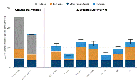
Lifecycle greenhouse gas emissions for conventional and electric vehicles in grammes CO2-equivalent per kilometre, assuming 150,000 kilometres driven over the vehicle lifetime. The error bars show a range of values for emissions from battery manufacture. 

Air Pollution Costs and Emission Reduction Targets

Various studies have monetized (measured in monetary units) air pollution costs, taking into account the types of pollutants, the harms they impose and the degree of human exposure (CE Delft 2019; Litman 2009; Shindell 2015; Wolfe 2019).

A growing body of research is investigating how pollution exposure affects health, taking into account the distance between emission sources and lungs, and the amount of pollution that people actually inhale, as summarized in the box below.

Air pollution costs (per ton of emission) are higher where population densities are high, Several studies indicate that automobile occupants are exposed to more harmful air pollution than people traveling by other modes, but pedestrians and cyclists inhale more air per minute and so may be exposed to greater risk (NZTA 2011). Some demographic groups, such as children, seniors and people with allergies, are likely to experience more harm from a given level of air pollution exposure.

Emission and Vehicle Travel Reduction Targets

Most jurisdictions in the world have emission reduction targets. For example, under the 2015 Paris Agreement, the United States committed to reducing its greenhouse gas (GHG) emissions by 26-28% between 2005 and 2025, and some jurisdictions have more ambitious goals, such as California�s commitment to reduce 1990 emissions 40% by 2030 and 80% by 2050. Britain is committed to reduce GHG emissions 100% (called net zero) by 2050.

Many jurisdictions are establishing goals and targets to reduce automobile travel and increase use of resource-efficient modes. For example, California has targets to reduce vehicle travel by 15%, increase walking, bicycling, and public transit, and achieve 10-15% active mode share in major transit hubs. Washington State law has a target to reduce per capita vehicle travel by 30% by 2035 and 50% by 2050. These targets help coordinate efforts by various levels of government and organizations to support walking, bicycling and public transit travel, and implement TDM and Smart Growth policies. For example, California is changing the way that transportation and land use development projects are evaluated from �LOS to VMT,� meaning that, rather than assuming that the planning goal is to maximize roadway level-of-service (LOS) and therefore traffic speeds, the new goal is to minimize vehicle miles of travel (VMT).

Comparing Emission Reduction Strategies

There are two general ways to reduce vehicle air pollution emissions: cleaner vehicle strategies which reduce emission rates per vehicle-kilometre, and Transportation Demand Management (TDM) strategies which reduce total vehicle travel (Litman 2005; Small 2019). Table 3 lists common examples of these strategies.

Table 3����������� Summary of Emission Reduction Strategies

Clean Vehicles (Reduce Emission Rates)

TDM (Reduce Vehicle Travel)

Promote use of efficient or alternative fuel (e.g., hybrid, electric and hydrogen) vehicles Anti-idling Emission standards Feebates Fuel efficiency standards Fuel quality improvements Inspection and maintenance (i/m) programs Low and zero emission vehicle mandates Neighborhood vehicles Resurface highways Roadside �high emitter� identification Scrapage programs Transit emission reduction programs

More multimodal planning (more support for walking, bicycling, public transit, ridesharing, etc.) Reduced fuel subsidies, increased fuel taxes, and carbon taxes More efficient road and parking pricing Distance-based vehicle insurance and registration fees TDM programs (commute trip reduction, freight transport management, etc.) Smart Growth policies that result in more compact and mixed development Reduce parking minimums

This table identifies various types of emission reduction strategies, including �clean vehicle� strategies that reduce emission rates, and Transportation Demand Management (TDM) strategies that reduce total vehicle travel.

There is considerable debate con concerning which approach is best overall. Some studies (McKinsey 2007; Project Drawdown) assume that clean vehicle strategies are more effective and cost effective than vehicle travel reduction strategies, but this generally reflects incomplete analysis. Such studies are generally performed by engineers and economists with little knowledge of TDM and Smart Growth strategies, and the analysis tends to consider a limited range of impacts. Many people are skeptical that TDM strategies can significantly reduce emissions. Most individual TDM strategies have modest impacts, affecting a small portion of total vehicle travel, but their impacts are cumulative and synergistic. An integrated TDM program can often reduce 20-30% of automobile travel where it is applied, and more if implemented with Smart Growth development policies.

Clean Vehicle strategies tend to provide just one or two types of benefits, primarily energy conservation and emission reductions, while TDM strategies tend to provide a much larger range of benefits, often called co-benefits (IGES 2011; IPCC 2014; Rashidi, Stadelmann and Patt 2017). In fact, because efficient and alternative fueled have lower operating costs, they tend to be driven more annual miles, a rebound effect, that increases other external costs including traffic congestion, road and parking infrastructure, crash risk, and non-tailpipe pollution (e.g., tire and road dust). Table 4 compares these impacts.

Table 4����������� Comparing Strategies (Litman, 2016)

Planning Objective	Efficient and Alternative Fuel Vehicles	TDM Solutions
Congestion Reduction	-	+
Parking Cost Savings	-	+
Facility Costs Savings	-	+
Consumer Costs Savings		+
Reduced Traffic Accidents	-	+
Improved Mobility Options		+
Energy Conservation	+	+
Pollution Reduction	+	+
Physical Fitness & Health		+
Land Use Objectives	-	+
Community Livability		+

Some transport improvement strategies help achieve one or two objectives (+), but by increasing total vehicle travel contradict others (-). TDM strategies reduce total motor vehicle travel, and so support many planning objectives, providing multiple economic, social and environmental benefits.

Compared with clean vehicle strategies, TDM strategies tend to provide these additional benefits:

• Social equity benefits, including affordability and more independent mobility for non-drivers.
• Reduced traffic congestion.
• Road and parking infrastructure cost savings.
• Consumer savings.
• Increased traffic safety.
• Improved public fitness and health.
• Reduced sprawl, which improves accessibility, reduced impervious surface area, and protects habitat.
• Improved community livability due to reduce neighborhood traffic and improved walkability.

TDM solutions have two additional benefits over cleaner vehicle strategies. First, many TDM strategies can be implemented much more quickly than changing the vehicle fleet. Although many vehicle manufactures are starting to produce electric vehicles, the technology is still relatively new with high prices, few models (particularly for SUVs, light trucks and vans), and operational obstacles such as limited recharging stations. In 2020 less than 5% of North American vehicle sales were electric. Optimistically, they may represent half of new vehicle purchases by 2030, but because only about 5% of the vehicle fleet is replaced each year, it typically takes one or two decades for new technologies to become dominant in the vehicle fleet, so at this rate it will take until the 2040s before most vehicle travel is electric.

In contrast, many TDM strategies can be implemented within a few years. Quick implementation strategies include Fuel Tax Increases, Carbon Taxes, efficient Parking Pricing, and other pricing reforms, Active Transport Planning� that significantly improves walking and bicycling (including e-bike) conditions, and Commute Trip Reduction and School Transport Management programs. Smart Growth policy reforms that allow significantly more infill development can also start to quickly reduce emissions by affected households.

Second, TDM programs tend to be much more equitable. Hybrid and electric vehicle purchase subsidies, subsidies to develop recharging stations, and a lack of road user taxes on electric vehicle use provide thousands of dollars in benefits to the affluent households that can afford such vehicles. In contrast, many TDM strategies directly benefit physically, economically and socially disadvantaged people by improving affordable and accessible mobility options (better walking, bicycling, ridesharing and public transit services), providing financial benefits such as Parking Cash-Out, and by reducing external costs, such as congestion, risk and pollution, that vehicle traffic imposes on other people.

Active and Micro Modes as Emission Reduction Strategies

Active (walking, bicycling and their variants) and motorized micro modes (e-scooters, e-bikes and their variants) could provide significant emission reductions, plus many other benefits. However, current emission reduction planning overlooks or undervalues this potential in favor of inefficient and inequitable electric car subsidies. Let�s consider what that means.

According to the National Household Travel Survey approximately 12% of total personal trips in the U.S. are made by active modes, but their potential use is much greater (Kuzmyak and Dill 2012). Approximately a quarter of all these trips are one mile or less, suitable for a twenty-minute walk; half of all vehicle trips are three miles or less, suitable for a twenty-minute bike ride; and most trips are less than five miles, suitable for a twenty-minute e-bike ride (Bhattacharya, Mills, and Mulally 2019). They estimate that a modest public investment in active transportation networks can deliver $74-138 billion in annual value, taking into account user savings, public health, economic growth and opportunity, and environmental quality. Surveys indicate that many people want to use these modes more often, for enjoyment, health, and affordability (NAR 2017).

E-scooters and e-bikes can overcome some obstacles to active travel: they can travel faster, carry heavier loads, and climb steeper inclines than human-powered modes, and are suitable for suburban conditions with longer travel distances. These modes tend to leverage additional vehicle travel reductions, so each mile of travel by active and micro modes can provide more than one reduced vehicle-mile. This occurs because users of these modes often choose closer destinations, for example, walking, scooting or biking to a local store rather than driving across town to a regional store, they reduce chauffeuring trips that often include empty backhauls, they provide access to public transit.

With sufficient facility improvements and incentives, active and micro modes can significantly reduce automobile travel. A major academic study, A Global High Shift Cycling Scenario, estimated that improving bicycle and e-bike conditions could increase urban bicycling mode shares from the current 6% up to 17% in 2030 and 22% in 2050 (Mason, Fulton and McDonald 2015). Other studies in North America (McQueen, MacArthur, and Cherry 2020) and Europe (Bucher et al. 2019) estimate that, accounting for various climatic and geographic constraints, e-bikes could achieve 10-15% mode shares and produce up to 12% emission reductions in typical urban areas. One Dutch survey found people who purchase an e-bike significantly increased their daily bicycle-kilometers and reduced their daily automobile-kilometers by 10% (Fyhri and Sundf�r 2020).

Despite the significant potential benefits, active and micro modes receive little attention in most emission reduction plans. Many jurisdictions provide thousands of dollars in subsidies to purchase a �zero emission� electric car, many jurisdictions are spending millions of dollars to create electric vehicle recharging stations, most jurisdictions accept hundreds of dollars in annual road subsidies per electric vehicle (since they don�t pay fuel taxes), and many provide preferred parking for electric vehicles. �Although active and micro modes also produce zero emissions, they receive far less support per vehicle-mile or vehicle-year; they are treated as an afterthought, to be considered after major policy decisions are made and supported with remaining resources.

Of course, increasing active and micro mode travel requires more than simply subsidizing scooters, bikes and e-bikes, it will require communities to make significant investments in facilities, TDM programs to encourage their use, and Smart Growth development policies that allow more affordable infill in order to create more compact neighborhoods. Although these are ultimately much cheaper than the facilities required for automobile travel, they require new money, while roads and parking facilities for automobiles have dedicated funds that require no public review. A level playing field would invest in active and micro mode improvements whenever they are cost-effective compared with automobile facilities, considering all costs, but this is seldom done, resulting in automobile-oriented solutions, and underinvestment in active and micro modes, TDM and Smart Growth.

This is inefficient, because electric vehicle subsidies have high costs per unit of reduced emissions, and because those vehicles tend to be driven more annual miles, which exacerbates traffic problems. It is also inequitable, because it results in huge subsidies that only directly benefit new vehicle purchasers, with no comparable benefit to people who cannot or prefer not to own an automobile.

Currently, U.S. governments spend more than $800 annually on roads for each motor vehicle, about half of which is funded through general taxes, and require businesses to provide off-street parking that totals an estimated $2,000-4,000 per vehicle year. Walking and bicycling have much lower facility costs per mile travelled, and since non-drivers travel far fewer annual miles than motorists, their facility costs and subsidies are far lower, by at least an order of magnitude. As a result, TDM policies that help households shift from driving to active and micro modes, and own fewer vehicles, provide huge infrastructure savings to governments and businesses.

This suggests that there is no lack of emission reduction strategies or resources to implement them; active and micro modes, and public transit are not only energy efficient and less polluting, they are also much cheaper for users, governments and businesses overall. What we lack is a planning process that prioritizes resource-efficient over resource-intensive travel.

This is not to suggest that active and micro modes can by themselves solve climate change; they are simply one of many potential emission reduction strategies. However, this is a good example of how conventional planning and funding practices favor automobile subsidies while under-investing in more cost-effective TDM solutions.�

As a result, more comprehensive analysis tends to increase support for TDM solutions. In addition, conventional traffic models tend to underestimate TDM impacts, so modelling improvements that reflect the additional vehicle travel caused by clean vehicle strategies, and the large vehicle travel reductions provided by integrated TDM programs, tend to justify more TDM solutions.

Skepticism concerning TDM effectiveness and benefits often reflects the assumption that, since vehicle travel provides benefits, vehicle travel reductions are difficult and harm consumers (Litman 2019). However, consumer surveys (NAR 2018) indicate that, although few motorists want to forego driving altogether, many would prefer to drive less, spend less money on transportation, rely more on other modes, provided that they are convenient, comfortable and affordable to use. TDM and Smart Growth help respond to those demands, increasing consumer welfare in addition to achieving community goals, including road and parking infrastructure savings, affordability, more independent mobility for non-drivers (and therefore social equity goals), improved public health and safety, plus environmental protection.

Demand Management Strategies

The following TDM strategies tend to be particularly effective at reducing energy consumption and pollution emissions.

Fuel Tax Increases and Carbon Taxes

Fuel Taxes are often considered a road user fee, which can be increased to recover more roadway costs. Carbon Taxes are taxes based on fossil fuel carbon content, and therefore a tax on carbon dioxide emissions. Fuel tax increases are an effective way to reduce energy consumption and carbon emissions, but is less effective at reducing other emissions or other mileage-related costs. One of the most appropriate emission reduction strategies is to eliminate current fuel subsidies (Koplow 2010).

Raising fuel price has two effects, it causes modest reductions in vehicle mileage, and over the long term encourages motorists to choose more fuel-efficient vehicles. A 10% price increase typically reduces fuel consumption by about 3% within one year and 7% over a five to ten year period (Elasticities). About one-third of the long-term energy savings result from reduced driving, and about two-thirds results from consumers shifting to more fuel-efficient vehicles.

It is uncertain how much increased fuel efficiency reduces emissions other than CO₂. Manufactures design vehicles to meet specific emission standards, and so implement more control strategies in vehicles with larger engines than in vehicles with smaller engines. Some emission control strategies reduce fuel efficiency (for example, catalytic converters add weight, and tuning engines to minimize NOx emissions increases fuel consumption). Reducing vehicle weight and wind resistance tends to reduce non-tailpipe emissions such as tire particles and road dust, but these effects are difficult to quantify. Most emissions decline in proportional to mileage.

Since taxes represent about half of total fuel prices in North America, a 20% tax increase is required to produce a 10% price increase. Fuel prices can be increased through Market Reforms such as a revenue-neutral tax shift (increasing fuel taxes and using the revenue to reduce other taxes that are considered more economically harmful, such as taxes on employment and business activity). Such tax shifts can provide Economic Development benefits by reducing employment and investment costs, reducing the economic costs of imported petroleum, stimulating energy efficiency technological innovation, and encouraging consumers to shift their expenditures to goods that generate greater regional employment (Goldstein, 2007). Shapiro, Pham and Malik (2008) used the U.S. Department of Energy�s National Energy Modeling System (NEMS) to evaluate the economic impacts of a carbon tax that begins at $14 per ton of CO2 equivalent and increases to $50 per ton, with 90% of the revenues returned to households and businesses in tax relief and the remaining 10% of revenues used to support energy and climate-related research and development, and new technology deployment. They conclude that this can reduce climate change emissions by 30% while only reducing 2010-to-2030 GDP growth from 33.6% to 33.4%.

Distance-Based Emission Fees

Distance-Based Emission Fees are mileage-based charges that reflect a vehicle�s emission rate. For example, an older vehicle that lacks current emission controls might pay 5� per mile, while a newer vehicle might pay 1�, and an Ultra-Low Emission Vehicle might pay 0.2�. This gives motorists with higher polluting vehicles a greater incentive to reduce their mileage, and conversely, gives motorists who drive high mileage a greater incentive to choose low polluting vehicles. Fees can vary depending on when and where driving occurs, with higher charges at times and locations where pollution impacts are greater (Pricing Methods). A more advanced system uses electronic sensors to measure actual tailpipe emissions when a vehicle is driven, giving motorists an incentive to minimize emissions in a variety of ways: choosing less polluting vehicles, reducing mileage, keeping engines well-tuned, and driving more smoothly.

Pay-As-You-Drive Vehicle Insurance and Other Distance Based Fees

Pay-As-You-Drive (PAYD) pricing means that fixed vehicle fees such as insurance and registration charges are converted into variable fees. For example, a motorist who now pays $1,000 per year for insurance would instead pay about 8� per mile, which gives motorists a new opportunity to save money if they driving less. Other fees, such as vehicle registrations, licensing, taxes and lease fees can also be made distance-based.

PAYD pricing can provide a variety of benefits:

� Increased equity (fees more accurately reflect the costs imposed by each vehicle).

� Increased affordability (motorists can minimize their insurance and registration fees by minimizing their mileage, which is not currently possible).

� Reduced uninsured driving (increased affordability can help lower-income and low-annual mileage motorists afford insurance coverage).

� Reduced crash risk (reduced mileage reduces crashes, and PAYD insurance gives higher-risk motorists the greatest incentive to reduce their mileage).

� Reduced traffic congestion.

� Road and parking costs savings.

Converting vehicle insurance and registration fees to PAYD approximately doubles variable vehicle expenses. This is predicted to reduce vehicle travel by approximately 10%, or 12% if vehicle registration fees are also distance-based. Because this involves changes to existing vehicle charges rather it should face less political opposition than a new fee or tax. It can be implemented as consumer option (just as consumers are able to choose a telephone or Internet service rate structure).

Freight Transport Management

Freight and commercial transport represents about 40% of transportation energy consumption, and a somewhat smaller but still significant portion of pollution emissions. Diesel freight vehicles tend to produce high particulate and sulphur emissions, although, as described earlier, these are declining as more rigorous emission control standards are implemented. Some studies estimate that freight energy efficiency can realistically increase by 15-30% over a 10-20 year period (OECD/IEA, 2001, p. 157). The specific strategies described below can increase freight efficiency and reduce pollution.

� Increase freight vehicle fuel efficiency and reduce emissions through design improvements and new technologies. These include increased aerodynamics, weight reductions, reduced engine friction, improved engine and transmission designs, more efficient tires, and more efficient accessories.

� Encourage shippers to use more energy efficient modes, such as rail and water transport rather than trucking for longer-distance shipping.

� Improve rail and marine transportation infrastructure and services to make these modes more competitive with trucking. (Note that by reducing shipping costs this may increase total freight traffic volumes, resulting in little or no reduction in energy consumption, emissions or other externalities.)

� Improve scheduling and routing to reduce freight vehicle mileage and increase load factors (e.g., avoiding empty backhauls). This can be accomplished through increased computerization and coordination among distributors.

� Organize regional delivery systems so fewer vehicle trips are needed to distribute goods (e.g., using common carriers that consolidate loads, rather than company fleets).

� Reduce total freight transport by reducing product volumes and unnecessary packaging, relying on more local products, and siting manufacturing and assembly processes closer to their destination markets.

� Use smaller vehicles and human powered transport, particularly for distribution in urban areas.

� Implement fleet management programs that increase system efficiency, use optimal sized vehicles for each trip, and insure that fleet vehicles are maintained and operated in ways that minimize pollution emissions.

� Encourage retrofit or scrapping of older, higher-polluting freight vehicles.

� Increase land use Accessibility by Clustering common destinations together, which reduces the amount of travel required for goods distribution.

� Pricing and tax policies to encourage efficient freight transport.

� Improve vehicle operator training to encourage more efficient driving.

Aviation Transport Management

Aviation is a major source of energy consumption and pollution emissions, is one of the fastest growing transportation sectors, has relatively high fuel consumption rates per passenger-mile (see Table 2), and tends to stimulate increased travel. High altitude air pollution emissions by jets tend to impose particularly high greenhouse impacts, and aircraft cause local air and noise pollution problems. Aviation represents about 10% of current transportation energy consumption.

Although some air travel is relatively inelastic (which is why airlines can sell high-priced business-class seats), much air travel is highly price sensitive (which is why airlines offer discounted fares), so even modest price increases can reduce air travel. Since fuel represents about 10% of total air travel costs, this suggests an elasticity of air travel with respect to total operating costs of about �1.0 or greater. Various policies and management strategies can encourage more efficient, less polluting air travel, and shifts to other modes, particularly to rail and bus for medium-distant trips (200-800 miles). These include:

� Eliminate airport infrastructure property tax exemptions, and increase aviation fuel tax rates. Eliminate duty-free shops at airports.

� Increase airport user fees to provide full cost recovery of airport infrastructure investments, air traffic controls and security services.

� Support development of fast and efficient rail transport on busy corridors to compete with air transport for medium-distance journeys.

� Upgrade and replace older aircraft with newer models that reduce fuel consumption, noise and air pollution emissions.

� Improve air traffic management systems to increase operational efficiency.

TDM Programs

Various types of programs implement specific TDM services within a particular geographic areas or group. Many TDM strategies need such a program to be implemented. Such a program has stated goals, objectives, a budget, staff, and a clear relationship with stakeholders. It may be a division within a transportation or transit agency, an independent government agency, or a public/private partnership. Below are examples.

Table 5����������� TDM Programs

Program Type	Scope	Travel Affected
Commute Trip Reduction (CTR) Programs	Employees in a particular business or jurisdiction.	Commute trips (about 25% of personal travel).
Transportation Management Association	Employees, businesses and clients in a district or jurisdiction.	Personal and some freight travel within an area.
Campus Transport Management	Serves students, staff and visitors in a college, university or research campus.	Commutes, and sometimes other trips.
School Transport Management	Serves students, parents and staff within a school.	School trips (about 5% of personal travel).
TDM Programs	Businesses, employees, residents and visitors within a district or jurisdiction.	Travel in the affected area.
Tourist Transport Management	Visitors, businesses and staff.	Travel in resort areas. Any leisure travel.
Special Event Transport Management	Participants and staff at special events, and travelers during emergencies.	Affected travel.

TDM programs typically include some of the following strategies:

� Commuter Financial Incentives (Parking Cash Out and Transit Allowances).

� Rideshare Matching.

� Parking Management and Parking Pricing.

� Alternative Scheduling (Flextime and Compressed Work Weeks).

� Telework.

� TDM Marketing and Promotion.

� Guaranteed Ride Home.

� Walking and Cycling Encouragement.

� Walking and Cycling Improvements.

� Bicycle Parking and Changing Facilities.

� Land use planning that reflects Location-Efficient Development principles.

� On-site amenities such as childcare, restaurants and shops, to reduce the need to drive for errands.

Market Reforms

A number of Transportation �and Land Use market reforms can help reduce energy consumption and pollution emissions, and encourage more efficient land use. These include:

� Full cost pricing (also called marginal cost pricing), which means that users pay directly for costs imposed on society by their vehicle use. This can include direct road user fees, parking pricing, insurance pricing reforms, tax reforms (for example, charging property taxes on road rights-of-way), and vehicle emission fees.

� Revenue-neutral tax shifts. Since governments must tax something to raise revenue, many economists recommend shifting taxes from socially desirable activities to activities that impose external costs. For example, fuel taxes and other road user charges could increase, and the revenues used to reduce employment and business taxes.

� More neutral tax policies. Some current tax policies unintentionally favor automobile use. For example, tax policies encourage employers to provide company cars or offer generous mileage reimbursement rates as a perk, and parking is often taxed at a lower rate than other goods.

� Least-Cost Transportation Planning. Least-Cost Planning means that demand management strategies are given equal consideration as capacity expansion in planning and funding.

� Cost-based development and utility fees. Clustered development tends to have lower public service costs, but these savings are not generally reflected in development and utility fees. More cost-based pricing can encourage more infill development.

� Improved transportation pricing methods. Conventional parking pricing and road tolling systems are inconvenient and expensive to operate. New Pricing Methods can overcome these problems, making direct user charges more feasible and politically acceptable.

There is virtually no technical limit to how much these strategies can reduce transportation energy consumption and emissions, their barriers are primarily political and institutional. Transportation market reforms justified on efficiency grounds (such as more efficient pricing of roads, parking and vehicle insurance) could reduce VMT by about one third, plus additional long-term travel reductions from more efficient land use development patterns (Litman 2014).

Land Use Management Strategies

Land use management strategies such as Smart Growth, New Urbanism, Transit Oriented Development, and Location-Efficient Development can reduce per capita automobile use, transportation energy use and emissions by improving Accessibility and Transportation Options.

For example, Salon (2014) used detailed travel survey data to analyze how demographic and geographic factors affect travel activity, and developed models for predicting how various land use development changes will affect travel, as illustrated below. Decker, et al. (2017) used Salon�s model to estimated that policies that encourage urban infill could reduce a region�s average household travel by about a third, from 57 down to 39 average daily vehicle-miles.

Figure 2��������� Household Vehicle Travel by Location (Salon 2014)

Per capita motor vehicle travel and emissions are much lower (20-60%) in compact, transit-oriented than in sprawled, auto-dependent areas.

Land use reforms can provide a number of benefits (Land Use Evaluation). Increased land use density and mix tend to reduce total per capita emissions (Boarnet and Handy 2010; Lawrence Frank and Company 2005; TRB 2009), although it can increase exposure to local emissions such as carbon monoxide, particulates and noise. Ewing, et al. (2007), provide detailed analysis of the ability of Smart Growth land use policies to reduce emissions; they estimate the cost effective land use changes can provide energy conservation benefits comparable to shifting average motorists to hybrid vehicles, while providing other economic, social and environmental benefits. In a study comparing per capita carbon emission rates by U.S. metropolitan regions, Sarzynski, Brown and Southworth (2008) found that �density, concentration of development, and rail transit all tend to be higher in metro areas with small per capita footprints. Much of what appears as regional variation may be attributed to these spatial factors.�

The following land use factors can affect energy consumption and emissions (Land Use Impacts on Transportation):

� Density (the number of people and businesses in a given area) and Clustering (common destinations located close together) affects the distances that people must travel, and the potential of transit, walking and cycling.

� Land use mix (the diversity of land uses in an area) affects trip distances and the feasibility of nonmotorized transportation.

� Major activity centers (locate employment, retail and public services close together in walkable commercial centers) increases the feasibility of transit use and allows people to make personal and business errands without driving.

� Parking management (flexible minimum parking requirements, shared parking, priced parking and regulations to encourage efficient use of parking facilities) affects the relative price and convenience of driving, and affects land use density, accessibility and walkability.

� Street connectivity (the degree to which streets connect to each other, rather than having deadends or large blocks) affects accessibility, including the amount of travel required to reach destinations and the relative speed and convenience of cycling and walking.

� Transit Oriented Development (locating high-density development around transit stations) makes transit relatively more convenient, and can be a catalyst for other land-use changes (CNT 2010).

� Pedestrian Accessibility (walkability) and Traffic Calming (roadway design features that reduce traffic speeds) affect the relative speed, convenience and safety of nonmotorized transportation.

Although individually each of these factors has relatively modest travel impacts, residents of traditional communities that incorporate most or all of these factors tend to drive 20-40% less than otherwise comparable residents of automobile-dependent communities (Land Use Impacts on Transport).

Nonmotorized Transportation Improvements and Encouragement

Shifts from automobile to nonmotorized transportation can be particularly effective at energy conservation and emission reductions by reducing short motor vehicle trips which have high per-mile fuel consumption and emission rates. As a result, each 1% shift of mileage from automobile to nonmotorized modes tends to reduce energy consumption and pollution emissions by 2-4%. A short pedestrian or cycle trip often replaces a longer automobile trip (for example, consumers may choose between shopping at a local store or driving to a major shopping center). Nonmotorized transportation improvements are also important for increasing transit use and creating more Accessible land use patterns.

Petritsch, et al. (2008) develop a model for predicting the mode shifts and energy savings likely to result from the addition of a particular cycling facility. According to some estimates, 5-10% of urban automobile trips can reasonably be shifted to non-motorized transport (Pedestrian Improvements). Walking and cycling improvements can help reduce total travel: a short walking or cycling trip replaces a much longer automobile trip, and nonmotorized travel improvements support transit use and more accessible development patterns. Some pedestrian-friendly communities have 5-10 times as many nonmotorized trips as occurs in more Automobile Dependent communities with otherwise similar demographic and geographic conditions.

Frank, et al. (2011) used detailed data on various urban form factors to assess their impacts on vehicle travel and carbon emissions. Their analysis indicates that increasing sidewalk coverage from a ratio of 0.57 (the equivalent of sidewalk coverage on both sides of 30% of all streets) to 1.4 (coverage on both sides of 70% of all streets) could reduce vehicle travel 3.4% and carbon emissions 4.9%. Based on the study results the team developed and tested a spreadsheet tool that can be used to evaluate the impacts of urban form, sidewalk coverage, and transit service quality and other policy and planning changes suitable for neighborhood and regional scenario analysis.

Ridesharing.

Ridesharing refers to carpooling and vanpooling. Carpooling uses participants� own automobiles. Vanpooling uses vans that are usually owned by an organization (such as a business, non-profit, or government agency) and made available specifically for commuting. Vanpooling is particularly suitable for longer commutes (10 miles or more each way). Ridesharing can be the most cost effective transportation mode. Carpooling that makes use of existing vehicle seats that would otherwise travel empty have very low incremental costs. Vanpooling with 6 or more passengers in a vehicle tends to have the lowest average cost per passenger-mile, since it carries more passengers per vehicle than a carpool, and does not require a professional driver or empty backhauls like conventional public transit services.

There are several ways to support and encourage ridesharing, including providing rideshare matching and vanpool organizing services, Marketing, Commuter Financial Incentives and HOV Priority.

Road Pricing

Road Pricing means that motorists pay directly for using a particular roadway or driving in a particular area. Road Pricing can be implemented as a demand management strategy, to fund roadway improvements or for a combination of these objectives. Economists have long advocated Road Pricing as an efficient and equitable way to pay roadway costs and encourage more efficient transportation. Below are specific types of road pricing

� Toll Roads are a common way to fund highway and bridge improvements. This is considered more equitable and economically efficient than other roadway improvement funding options.

� Congestion Pricing (also called Value Pricing) refers to road pricing used to reduce peak-period vehicle travel.

� High Occupancy Toll (HOT) lanes are High Occupancy Vehicle lanes that also allow access to low occupancy vehicles if drivers pay a toll. This allows more vehicles to use HOV lanes while maintaining an incentive for mode shifting, and raises revenue.

� Cordon (Area) Tolls are fees paid by motorists for driving in a particular area, usually a city center during weekdays. This can be done by simply requiring vehicles driven within the area to display a pass, or by tolling at each entrance to the area.

� Vehicle Use Fees such as mileage-based charges can be used to fund roadways and reduce vehicle travel (Distance-Based Fees).

Transit Improvements and Incentives

A variety of strategies can encourage transit use, including increased service, more convenient and comfortable service, transit priority traffic management, lower fares, improved marketing, commuter incentives (such as employee transit benefits), improved pedestrian and bicycle access to transit stops, and Transit Oriented Development. In most communities, 5-10% of automobile trips could shift to transit if these strategies are widely implemented.

Transit consumes less energy and produce less pollution per passenger-mile than automobile travel, and people who rely on transit tend to travel fewer passenger-miles than motorists, so increased transit tends to reduce per capita energy consumption and pollution emissions. A variety of factors affect the energy conservation and emission reduction impacts of transit improvements and incentives (Transit Evaluation). A full transit vehicle consumes less than 10% of the energy per passenger-mile as automobile travel, but in practice system-wide energy savings tend to be smaller due to relatively low load factors (transit vehicles often make trips with relatively few passengers).

Strategies that increase transit load factors (for example, fare discounts, more comfortable vehicles and better information, that increase ridership on routes that have excess capacity) can provide significant emission reductions. Transit improvements can provide a catalyst for broader travel and land use change. For example, people who commute by transit do not usually drive for errands during their breaks, and attractive transit service may allow some households to give up a second car, resulting in reduced per capita automobile travel. Transit Oriented Development helps create multi-modal communities where residents and employees drive less overall (Land Use Impacts on Transport). Some research indicates that each passenger-mile of rail travel represents 3 to 6 miles of reduced automobile travel if a transit system provides a catalyst for more accessible land use, suggesting that total energy saving and emission reduction benefits may be many times greater than what results directly from passenger-miles shifted from automobile to transit (Transit Evaluation).

Parking Management and Parking Pricing

Parking Management and Parking Pricing strategies are an effective way to reduce automobile travel, and tend to be particularly effective in urban areas where pollution problems are greatest. Charging motorists directly for the parking tends to reduce automobile trips by 10-30% of affected trips. Parking management and pricing supports use of alternative modes, improves walkability, and encourages more efficient land use.� Also, by reducing the total amount of pavement in an area they help reduce Heat Island Effects (increased ambient temperatures in paved areas) which tends to increase ozone (Gorsevski, et al, 1998).

TDM Marketing

TDM Marketing includes activities that provide consumer information and encouragement to support TDM. Marketing can have a major impact on TDM program effectiveness. Some TDM marketing programs have reduced automobile travel more than 10%.� TDM marketing includes:

� Educating public officials, businesses about TDM strategies they can implement.

� Informing potential participants about TDM options they can use.

� Identifying and overcoming market barriers to the use of alternative modes.

� Promoting benefits and changing public attitudes about alternative modes.

Traffic Calming and Roundabouts

Traffic Calming includes a variety of roadway design features that reduce vehicle traffic speeds and volumes. The energy and emission impacts depend on project design and conditions. Some Traffic Calming strategies result in smoother traffic and more optimal speeds, reducing energy consumption and emissions. In particular, Modern Roundabouts that replace stop signs and traffic signals can improve traffic flow (www.RoundaboutsUSA.com). Other Traffic Calming strategies increase stop-and-go driving and reduce traffic speeds below optimal vehicle efficiency (i.e., below 20 mph), and so may increase per-mile vehicle energy consumption and emissions. Impacts on per capita energy consumption and emissions depend on whether Traffic Calming reduces total vehicle travel by making alternative modes and more accessible urban neighborhoods relatively more attractive.

�Car-Free Planning and Vehicle Restrictions

Comprehensive Car-free Planning and Vehicle Restrictions can reduce vehicle use, energy consumption and emissions, if implemented as part of a comprehensive program to increase transportation and land use efficiency. If applied on a small scale, such as a single street or commercial centers, it may simply shift when and where driving occurs, causing little or no energy savings or emission reduction benefit. Some types of vehicle restrictions, such as no-drive days based on license plate numbers, are used during extreme air pollution emergencies, but are probably not effective as long-term strategies. Some households will even purchase a second car to use during their regular vehicle�s no-drive days, or rely on taxis rather than personal automobiles.

Telework

Telework involves the use of telecommunications to substitute for physical travel. This includes telecommuting, distance learning, and various forms of electronic business and government activities. According to some estimates up to 50% of all types of jobs are suitable for Telework, but the actual portion of trips that can be reduced by telework appears to be much lower, since many jobs require access to special materials and equipment, or frequent face-to-face meetings, and not all employees want to telework or have suitable home conditions. A portion of the reduced travel is often offset by additional vehicle trips teleworkers make to run errands, and because it allows employees to move further from their worksite, for example, choosing a home of job in a rural area or another city because they know that they only need to commute two or three days a week.

Speed Reductions

Traffic speeds reductions can reduce energy consumption and emissions in two ways. Lower speeds tend to reduce total vehicle mileage. The elasticity of vehicle travel with respect to travel time is� �0.2 to �0.5 in the short run and �0.7 to �1.0 over the long run, meaning that a 10% reduction in average traffic speeds reduces affected vehicle travel by 2-5% during the first few years, and up to 7-10% over a longer time period (Transport Elasticities).

In addition, vehicle fuel consumption and emissions tend to increase at speeds greater than 55 miles per hour, as indicated in figures 1 and 2. For a typical car, fuel efficiency declines about 1% for each additional mile above 55 mph. Reducing travel speeds from 65 to 55 mph provides about 10% fuel savings for a 1997 model vehicle, and about 18% for a 1984 model vehicle. Some researchers suggest that significant energy savings and emission reductions could be achieved by enforcing existing traffic speed limits (Suzuki, 1998).

Sustainable Transportation Planning

Sustainable Transportation refers to transportation systems that respond to long-term and indirect economic, social and environmental objectives. Global air pollution and depletion of non-renewable resources are major concerns for Sustainable Transportation. Sustainable Transportation planning can provide a framework for implementing energy conservation and emission reduction strategies.

Other Strategies

Energy conservation and emission reduction strategies that do not involve TDM are described below.

Promote Efficient and Low Emission Vehicle Purchases

Information and promotion can encourage consumers and fleet managers to purchase more efficient, less polluting vehicles. U.S. federal law requires vehicle manufacturers to post fuel efficiency ratings on new vehicles, and information resources such as those listed below can help consumers take energy and emission factors into account when selecting a vehicle.

ITF (2020), Good to Go? Assessing the Environmental Performance of New Mobility, International Transport Forum (www.itf-oecd.org); at https://bit.ly/34WWTAy.

This report compares lifecycle energy consumption and emissions from various vehicle types, including internal combustion, electric and hydrogen cars, plus taxi and ridesharing operations.

Fuel Economy Website (www.fueleconomy.gov), by the U.S. Department of Energy and the U.S. Environmental Agency provides information on fuel consumption ratings of new automobiles and additional information on vehicle efficiency strategies.

Emission Standards

These are requirements that manufacturers produce vehicles that incorporate certain technologies (such as emission catalysts) or meet a maximum emission standard. These have been widely applied and have been successful at reducing per-mile emission rates for some pollutants. Such standards can be increased to force manufactures to develop and implement additional emission controls.

Fuel Efficiency Standards

Corporate Average Fuel Efficiency (CAFE) standards require vehicle manufactures to produce and sell more fuel-efficient vehicles. Manufactures pay a fine if the vehicles they sell on average exceed these standards. The U.S. CAFE was 40.9 mpg in 2020 and increases 1.5% each year through model year 2026.

Gas Guzzler Taxes

A Gas Guzzler Tax is a special tax on the purchase of new vehicles based on their fuel consumption rates, to encourage the manufacture and sale of more fuel-efficient vehicles.

Feebates

Feebates are a surcharge on the purchase of new fuel inefficient vehicles, with the revenue used to provide a rebate on the purchase of fuel-efficient vehicles (Perrin, 2000). The table below indicates the predicted impact of Feebates, based on a 9-liters/100 kilometer base. For example, if a $500 level is used, a vehicle rated at 6 liters/100 km would receive a $1,500 rebate, while a vehicle rated at 11 liters/100 km would be charged a $1,000 fee. Kunert and Kuhfeld (2007) recommend a set of tax reforms to encourage the purchase of more fuel efficient vehicles.

Efficiency-Based Annual Registration Fees

An alternative to Gas Guzzler taxes or Feebates on the purchase of a new vehicle is an annual vehicle fee based on a vehicle�s fuel efficiency rating. This can be implemented by modifying the structure of existing vehicle registration fees rather than imposing a new fee. These may induce some motorists to purchase less polluting vehicles. Such fees tend to be regressive, since lower-income motorists are more likely to own a higher-polluting vehicle (Sevigny, 1998).

Transit Emission Reduction Programs

Transit vehicle emission reduction programs can be particularly cost effective because transit vehicles tend to drive high mileage under urban-peak conditions, and older diesel buses had high per-mile emission rates. Such programs include use of electric trolleys and alternative fuel buses (such as natural gas) to replace conventional diesel buses, retrofitting existing buses with cleaner diesel engines, and improving bus maintenance and operating practices (see USEPA �Urban Bus Retrofit/Rebuild� program at www.epa.gov/otaq/hd-hwy.htm).

Low and Zero Emission Vehicle Mandates

A Zero Emission Vehicle (ZEV) Mandate was created by California's Air Resources Board (CARB; www.arb.ca.gov) in accordance with Low-Emission Vehicle (LEV) Regulations passed in 1990. It requires that a portion of vehicles sold in California by major car companies be zero-emission (i.e., virtually no tailpipe emissions). Originally the mandate was to be 2% of vehicles in 1998, increasing to 10% in 2003, but in 1996, CARB changed the requirement to a �good faith effort� by manufactures to market ZEVs.

Inspection and Maintenance (I/M) Programs

This means that vehicles are inspected annually or biannually by a certified emission inspection station to identify those with excessive emission rates (www.epa.gov/otaq/cfa-air.htm). A typical I/M program fails about 10% of vehicles, which are required to be repaired or scrapped. Repairs resulting from I/M programs are estimated to reduce fleetwide vehicle fuel consumption by about 0.5%, emissions of NOx by 1%, hydrocarbons by 10% and carbon monoxide by 15%. As a larger portion of the vehicle fleet has modern engines with more durable emission controls, the effectiveness of such programs is expected to decline.

Roadside �High Emitter� Identification

Instruments are now available that identify the emission rates of vehicles as they drive pass a sensor (FEAT Data Center, www.feat.biochem.du.edu; MDNR 2005). These can be used with voluntary systems (see box below) or legal enforcement to have high emitting vehicles corrected. Some programs encourage police and citizens to report vehicles that appear to emit excessive smoke (www.smokey.org.nz).

Scrapage Programs

These programs involve the purchase and disposal of older, higher-emitting vehicles (Dill 2004). This can reduce local pollution emissions, since older vehicles tend to have high emission rates, but does little to reduce energy consumption since older vehicles are on average no more fuel-efficient than new vehicles. Such programs can be set based on vehicle age (i.e., vehicles must be 15 years or older), or vehicles that fail an emission test could qualify. There are potential problems with such programs, since many of the vehicles may be scrapped soon anyway, and some residents may even purchase an older vehicle from another region so it can be purchased through the program. Li, Linn and Spiller (2011) conclude that such programs provide little and costly emission reductions.

Fuel Quality Improvements

Vehicle fuel quality (such as sulphur and heavy metal content) affects the amount of pollution produced per vehicle-mile (SOx, heavy metals, NOx, and particulates), and some fuel contaminants can degrade vehicle emission control equipment. Fuel quality improvements can reduce some pollutants, and may slightly increase vehicle efficiency (Perrin, 2000; Working Group 1 on Environmental Objectives, 2000). Many jurisdictions, including the United States, Canada and some individual states regulate fuel quality. California has been a leader is setting high fuel quality standards. Fuel quality can also be improved by imposing higher taxes on lower-quality fuels or fuels that have harmful additives. This approach has been successful in reducing the use of leaded fuel.

Emission Capping and Trading

Emission Capping places a limit on the total amount of pollution that may be produced in an area. Emission Trading is a market structure that involves allocating or selling pollution rights, and allowing those rights to be traded to allow the most cost-effective emission reduction strategies to be implemented (Albrecht 2000; Neiderberger 2005). For example, if ten factories each receive a 100-ton-per-year emission allocation, those that can reduce emissions at a lower cost can sell their rights to others that have a higher cost per unit of emission reductions.

Emission trading has been effective and efficient at reducing some emissions when there are a small number of emitters (e.g., a few factories), but most analysts conclude that emission trading as it is currently practiced is not practical for reducing transportation emissions, at least at an individual level. Emission trading may allow funding of specific transportation emission reduction programs. For example, discounts

Fleet Management and Driver Training

There are many ways to increase motor vehicle performance and efficiency through best management practices, including regular inspections and maintenance, and improved driver training (Sivak and Schoettle 2011). This is especially appropriate for large vehicle fleets, such as delivery trucks, taxis and vehicle pools (PHH 2001). The FleetSmart Program funded by Natural Resources Canada (http://fleetsmart.nrcan.gc.ca) provides information on industrial fleet management for efficiency and safety. The Energy Environment Excellence Fleet Management website (www.e3fleet.com) provides practical information for optimizing vehicle fleet fuel efficiency and environmental performance.

The Repair Our Air-Fleet Challenge (www.repairourair.org) works with fleets to reduce inefficient fuel consumption through:

� Idling reduction (commercial vehicles often idle a significant portion of their operating time)

� Speed management

� Cab heater alternatives

� Maintenance practices

� Driver efficiency

Anti-Idling

Idling vehicles produce air and noise pollution. FleetSmart (2001) encourages truck drivers to minimize idling. Some communities have passed anti-idling laws that limit how long a vehicle can sit with the engine operating when it is not being driven (CCS, 2001). Some organizations provide information and resources to help reduce unnecessary engine idling (www.climatechangesolutions.com/municipal/land/tools/idle.html and �(www.oee.nrcan.gc.ca/idling/home.cfm).

Resurface Highways

Reducing highway surface roughness through improved maintenance and using less flexible pavement surfaces such as concrete rather than asphalt can reduce fuel consumption by as much as 10% for heavy trucks, and by a smaller amount for lighter vehicles (TC 1999). However, most studies indicate that this is not a very cost effective way to increase fuel efficiency.

Policy Reforms and Incentives

Governments can implement various reforms and provide incentives for implementation of emission reduction strategies. For example, governments can implement Institutional Reforms such as Least Cost Transportation Planning and Smart Growth Fiscal Reforms within its own jurisdiction.

Governments can perform sustainability audits of its policies, investments and programs to identify how they affect Sustainability objectives, including energy and emission reductions. This process can help prioritize funding allocations and design policies and programs to help achieve sustainability.

Federal, state and provincial governments often provide funding to regional and local governments. Special funding programs can be available for projects that reduce transportation emissions (such as transit and nonmotorized transportation improvements), and all types of grants can be prioritized based on how well they support sustainability objectives. For example, infrastructure funding that encourage efficient transportation and Smart Growth can be given priority over projects which are otherwise equally beneficial, but do not support these objectives. Federal, state and provincial grants can give priority to communities that have efficient transportation and land use policies. Such incentives can motivate communities to implement their own Institutional Reforms and Smart Growth Fiscal Reforms. This can increase the cost effectiveness of infrastructure investments, since efficient transportation and land use policies can reduce unit costs of providing public services such as roads, water, sewage and schools, particularly over the long run.

Flextime

Flextime means that employees are allowed some flexibility in their daily work schedules. For example, rather than all employees working 8:00 to 4:30, some might work 7:30 to 4:00, and others 9:00 to 5:30. This shifts travel from peak to off-peak periods. By itself it provides no reduction in vehicle mileage, although it can help transit and rideshare commuters match schedules.

Road Capacity Expansion and Traffic Signal Synchronization

Road widening and traffic signal synchronization are sometime advocated as ways to reduce traffic congestion, and therefore energy consumption and pollution emissions (TRB 1995; Cobian, et al. 2009). However, research suggests that at best these provide short-term reductions in energy use and emissions which are offset over the long-run due to Induced Travel (Noland and Quddus 2006). Field test indicate that shifting from congested to uncongested traffic conditions significantly reduces pollution emissions, but traffic signal synchronization on congested roads provides little measurable benefit, and can increase emissions in some situations (Frey and Rouphail 2001). According to a study by the Norwegian Centre for Transport Research (T�I 2009):

�Road construction, largely speaking, increases greenhouse gas emissions, mainly because an improved quality of the road network will increase the speed level, not the least in the interval where the marginal effect of speed on emissions is large (above 80km/hr). Emissions also rise due to increased volumes of traffic (each person traveling further and more often) and because the modal split changes in favor of the private car, at the expense of public transport and bicycling.�

Table 6 summarizes roadway improvement emission impacts, including effects on emission rates per vehicle mile, increases in total vehicle mileage, and emissions from road construction and maintenance activities.

Table 6����������� Roadway Expansion Greenhouse Gas Emission Impacts (T�I 2009)

	General Estimates	Large Cities	Small Cities	Intercity Travel
Emission reductions per vehicle-kilometer due to improved and expanded roads.		Short term reductions. Stable or some increase over the long-term.	Depends on situation, ranging from no change to large emission increases.	Depends on situation. Both emission reductions and increases can occur.
Increased vehicle mileage (induced vehicle travel), short term (less than five years)	A 10% reduction in travel time increases traffic 3-5%	Significant emission growth	Moderate emission growth	Moderate emission growth
Increased vehicle mileage (induced vehicle travel), long term (more than five years)	A 10% reduction in travel time increases traffic 5-10%	Significant emission growth	Moderate emission growth	Moderate emission growth
Road construction and improvement activity	12 tonnes of CO2 equivalent for 2-lane roads and 21 tonnes for 4-lane roads.	Road construction emissions are relatively modest compared with traffic emissions.
Roadway operation and maintenance activity	33 tonnes of CO2 equivalent for 2-lane roads and 52 tonnes for 4-lane roads.	Road operation and maintenance emissions are relatively modest compared with traffic emissions.

This table summarizes roadway improvement emission impacts according to research by the Norwegian Centre for Transport Research.

Intelligent Transportation Systems

Intelligent Transportation Systems include the application of a wide range of new technologies, including driver information, vehicle control and tracking systems, transit improvements and electronic charging (see ITS Online and ITS America). These can provide a variety of transportation improvements, including driver convenience, reduced congestion, increased safety, more competitive transit, and support for pricing incentives. ITE strategies that support transportation demand management reduce total vehicle travel (such as transit improvements and electronic road pricing) can reduce energy consumption and emissions, but not strategies that make driving more convenient, or squeeze more vehicles onto existing roadways, because they are likely to increase vehicle traffic mileage and speeds.

Evaluating Energy Conservation and Emission Reduction Strategies

Several studies have attempted to compare and rank energy conservation and emission reduction strategies in terms of potential effectiveness and cost effectiveness, in order to identify the �best� option (McKinsey 2007; Project Drawdown 2020). Their conclusions vary significantly based on the assumptions that are used.

Many evaluations ignore Rebound Effects, particularly the tendency of motorists to increase their mileage when increased fuel efficiency reduces per-mile vehicle operating costs. A 10% increase in vehicle fuel efficiency typically results in a 20-30% increase in vehicle mileage, resulting in a 7-8% net energy savings. Ignoring this impact tends to overstate the emission reduction benefit of technical strategies that increase fuel efficiency.

Most evaluations focus on direct implementation costs and emission reduction benefits, ignoring most other costs and benefits. Such an approach may favor strategies that are cost-effective at reducing emissions, but increase other problems such as consumer costs, crash damages or traffic congestion. A more Comprehensive Evaluation Framework considers a broader range of impacts, and so will favor that emission reduction strategies that provide additional benefits, such as consumer cost savings, road safety and congestion reductions.

Table 7 discusses whether each strategy described in this chapter is likely to cause induced travel, and what additional benefits and costs it is likely to cause. Strategies that reduce perceived vehicle operating costs tend to induce additional vehicle travel, and so tend to increase traffic congestion, facility costs, crashes and urban sprawl. Strategies that increase perceived vehicle operating costs tend to reduce total vehicle travel, and so can provide benefits such as reduced congestion, facility costs, crashes, and urban sprawl. Some strategies also improve consumer choice and savings. The vehicle travel impacts of some strategies depend on how they are implemented.

Table 7����������� Summary of Rebound Effects and Additional Benefits

	Induced Vehicle Travel	Additional Impacts
Distance-Based Emission Fees	None. Increases per-mile vehicle costs.	Can help reduce congestion, road and parking facility costs, crashes and urban sprawl.
Fuel Tax Increases	None. Increases per-mile vehicle costs.	Can help reduce congestion, road and parking facility costs, crashes and urban sprawl.
Freight Transport Management	Depends on which strategies are used.	Depends on which strategies are used. Strategies that reduce vehicle traffic can reduce congestion, roadway costs and crashes.
Aviation Transport Management	Depends on which strategies are used.	Depends on which strategies are used. Strategies that reduce air travel can reduce airport congestion, consumer costs and crashes.
TDM Programs	Depends on which strategies are used.	Strategies that reduce vehicle traffic can reduce congestion, roadway costs and crashes.
Pay-As-You-Drive Vehicle Insurance	None. Increases per-mile vehicle costs.	Can help reduce congestion, road and parking facility costs, crashes and increased equity.
Land Use Management Strategies	None.	Depends. Can reduce crashes, increase transportation choices, reduce sprawl and increase community livability.
Nonmotorized Transportation Improvements	None.	Can reduce congestion, road and parking facility costs, sprawl, and increase transport choices and community livability.
Consumer Information	If it encourages motorists to purchase more fuel-efficient vehicles than they would otherwise it may cause some induced travel.	Depends. Improves consumer choice and financial savings.
Road Pricing	Generally none, unless it significantly increases total roadway capacity and automobile dependency.	Depends on the type of pricing and how revenues are used. Can reduce congestion, road and parking facility costs, crashes and sprawl.
Transit Improvements and Transit Vehicle Emission Reductions	None.	Can reduce congestion, road and parking facility costs, sprawl, and increase transport choices and community livability.
Rideshare Programs	May encourage longer commutes.	Can reduce congestion, road and parking facility costs, sprawl, and increase transport choices.
Parking Management	None.	Can reduce congestion, road and parking facility costs and sprawl.
Traffic Calming and Roundabouts	None.	Can reduce crash risk and increase community livability.
Vehicle Restrictions	None, unless it only applies to a small area and causes travel to shift elsewhere.	Can reduce congestion, road and parking facility costs, sprawl, and increase transport choices and community livability.
Telework	Possible. Telecommuters may take additional non-commute trips or move farther away from their worksite.	Reduces traffic congestion, crashes, road and parking facility costs and improves commuter choice and savings. May contribute to sprawl.
Emission Control Standards	Generally none, unless it also reduces vehicle operating costs.	Depends.
Fuel Efficiency Standards	Yes. Reduces vehicle operating costs and so tends to increase vehicle mileage.	Tends to increase traffic congestion, road and parking facility costs, crashes and sprawl.
Gas Guzzler Taxes	Yes. Reduces vehicle operating costs and so tends to increase vehicle mileage.	Tends to increase traffic congestion, road and parking facility costs, crashes and sprawl.
Feebates	Yes. Reduces vehicle operating costs and so tends to increase vehicle mileage.	Tends to increase traffic congestion, road and parking facility costs, crashes and sprawl.
Efficiency-Based Annual Registration Fees	Yes. Reduces vehicle operating costs and so tends to increase vehicle mileage.	Tends to increase traffic congestion, road and parking facility costs, crashes and sprawl.
Super-Efficient and Alternative Fuel Incentives	Yes. Reduces vehicle operating costs and so tends to increase vehicle mileage.	Tends to increase traffic congestion, road and parking facility costs, crashes and sprawl.
Motorcycle Encouragement	Probably. Reduces vehicle operating costs and so increase vehicle mileage.	Tends to increase crash injuries and deaths.� Often increases conventional air pollutants (since few motorcycles have emission control equipment). Reduces parking costs.
Low and Zero Emission Vehicle Mandates	Probably. Reduces vehicle operating costs and so increase vehicle mileage.	Tends to increase traffic congestion, road and parking facility costs, crashes and sprawl.
Inspection and Maintenance (I/M) Programs	Probably. May reduce vehicle operating costs by a small amount.	Uncertain. May increase traffic congestion, road and parking facility costs, crashes and sprawl, but impacts are likely to be small.
Roadside "Hig Emitter" Identification	Unlikely. May reduce vehicle operating costs by a small amount.	Minimal.
Scrapage Programs	Probably none.	May increase road safety by reducing the number of old vehicles on the roadway.
Fuel Quality Improvements	Uncertain. May increase fuel costs but increase fuel efficiency.	Uncertain. Probably minimal.
Emission Capping and Trading	Depends on how the program is implemented.	May involve TDM strategies.
Fleet Management	Uncertain. May reduce vehicle-operating costs and reduce vehicle mileage.	Depends on what measures are implemented.
Speed Limit Enforcement	None. Tends to increase per-mile time costs and so reduce total mileage.	Can reduce crashes and sprawl, and increase community livability.
Anti-Idling	Probably none.	Can increase community livability due to reduced local air and noise pollution.
Neighborhood Vehicles	None. Likely to reduce total vehicle mileage.	Mixed impacts. Likely to increase consumer choice and community livability.
Resurfacing Highways	Probably. Reduces vehicle operating costs and increases comfort.	May increase traffic congestion, road and parking facility costs, crashes and sprawl.
Flextime	Probably. Reduces traffic congestion, which is likely to induce vehicle travel.	Reduces peak-period traffic congestion.
Road Capacity Expansion/Traffic Signal Synchronization	Yes. Reduces traffic congestion and vehicle operating costs, inducing additional vehicle travel.	Likely to increase downstream traffic congestion, road and parking facility costs, crashes, sprawl and automobile dependency, particularly over the long-run.
Intelligent Transportation Systems	Depends on which are implemented.	Strategies that reduce congestion and increase vehicle speeds and volumes may increase some costs.

This table indicates whether a strategy is likely to induce additional vehicle travel by reducing per-mile vehicle operating costs, and other benefits and costs that it is likely to cause.

Best Practices

� Consider a wide range of energy conservation and emission reduction strategies.

� A good rule of thumb is that TDM strategies should receive at least as much investment as clean vehicle strategies, and can be expected to achieve half or more of emission reduction targets.

� When evaluating potential emission reduction strategies, consider impacts besides energy conservation and emission reductions, including effects on consumer costs and transportation choice, congestion, parking costs, road safety, equity and community livability.

� Use comprehensive modelling. Account for the rebound effects of strategies that reduce per-mile vehicle operating costs, and therefore the additional congestion, infrastructure costs, crash risk and sprawl that results.

� Develop integrated TDM and clean vehicle programs.

� Establish targets to reduce vehicle travel and increase use of resource-efficient modes.

Examples and Case Studies

Local Emission Reduction Modelling

Jones, Wheeler and Kammen (2018) quantify the potential of local policies and programs to meet aggressive GHG reduction targets using a consumption-based, high geospatial resolution planning model for the state of California. We find that roughly 35% of all carbon footprint abatement potential statewide is from activities at least partially within the control of local governments. The study shows large variation in the size and composition of carbon footprints and abatement opportunities by ∼23,000 Census block groups (i.e., neighborhood-scale within cities), 717 cities and 58 counties across the state. These data and companion online tools can help cities better understand priorities to reduce GHGs from a comprehensive, consumption-based perspective, with potential application to the full United States and internationally.

Paris Vehicle Travel Reductions (Reid 2020)

Paris Mayor Anne Hidalgo has won reelection in the French capital based on her commitment to turn the French capital into a myriad of compact neighborhoods where you can find everything you need within 15 minute walk or bike from home, creating a �city of fifteen minutes��or, Ville Du Quart D�Heure. The plans, which aim to transform Paris into a people-friendly city, build on Hidalgo�s �Plan V�lo� transport changes made during her current term of office, which has included removing space for cars and boosting space for cyclists and pedestrians. This includes plans for every street to have a cycle path, and for all of the city�s bridges to have protected cycleways. The space required to make Paris cyclist-friendly would mostly come at the expense of motoring. Under her plans Paris will remove 72% of its on-street car parking spaces, or about 60,000 of the 83,500 on-street parking spaces in Paris.

(There are 621,600 parking spaces in total in Paris, most of them are domestic ones or commercial car parks.)

Hidalgo�s victory will now allow these eco-friendly moves�and others�to go ahead. She has a six-year term of office and will be able to push through many if not all of the measures she has promised.

Active Transport in Britain

The UK Department for Transport�s report, Gear Change: A Bold Vision for Cycling and Walking, establishes a goal that by 2030, half of all journeys in towns and cities will be cycled or walked, in order achieve various benefits including improving health and wellbeing, reducing inequalities, improving air quality, combatting climate change, reducing traffic congestion and supporting local economic activity. The plan advocates significant investments in walking and bicycling facilities, urban planning reforms, and restrictions on car traffic in some areas, to support active transport. The vision includes these themes:

• There will be first hundreds, then thousands of miles of safe, continuous, direct routes for cycling in towns and cities, physically separated from pedestrians and volume motor traffic, serving the places that people want to go.
• Putting cycling and walking at the heart of transport, place-making, and health policy.
• Empowering and encouraging local authorities.
• We will enable people to cycle and protect them when they cycle.

50 Transportation Emission Reduction Strategies (Dutzik 2016)

The report, ), 50 Steps Toward Carbon-Free Transportation:� Rethinking U.S. Transportation Policy to Fight Global Warming, identifies fifty ways that public policies can encourage more energy efficient and lower-polluting transportation. It describes a New Transportation Toolbox of strategies that � especially if combined in ways that maximize synergies among them � can help to create a zero-carbon transportation system. Among those strategies are:

Repowering Vehicles: Efficient electric vehicles that can be powered by clean, renewable electricity are entering the marketplace faster than the hybrid cars of a decade ago, and technology continues to improve, reducing costs and increasing travel range. Electric vehicles reduce carbon emissions even when using electricity from today�s grid, and will deliver greater benefits in the years to come as America transitions to electricity provided by clean, renewable sources of energy.

Urbanization and Smart Growth: American cities � especially their downtowns � are experiencing a renaissance, driven by a growing desire for walkable living. A future in which most new development takes place in urban and walkable neighborhoods could reduce transportation greenhouse gas emissions by 9 to 15 percent by mid-century, according to research by the Urban Land Institute.

Shared Mobility: Over the last decade, an explosion of technology-enabled services � from carsharing to bikesharing to Lyft and Uber � has revolutionized transportation in many cities. Some of these �shared mobility� services have been shown to reduce vehicle ownership and driving, while the effects of others are just beginning to be studied.

Public Transportation: Transit ridership hit a modern high in 2014, the result of recent transit expansion projects and growing urban population and employment. Current public transportation services reduce vehicle travel (and greenhouse gas emissions) by about 10 percent in U.S. cities, according to research conducted for the Transportation Research Board.

Reallocating Space: The vast majority of street space in American cities is devoted to moving or storing cars, pushing people who walk, bike or take transit to the margins. Cities in the United States and around the world are reallocating space formerly devoted to cars to other public purposes, encouraging the use of low-carbon modes of transportation. U.S. cities with good bicycling infrastructure have nearly twice as many bike commuters as the national average.

Smart Pricing: Americans typically pay nothing to drive on most roads and enjoy the lowest gas taxes in the industrialized world. Government subsidies for driving and parking, along with free access to roads and policies that encourage annual pricing for auto insurance and other costs of driving, create economic signals that encourage Americans to drive and put competing low-carbon transportation modes at an economic disadvantage. Cities around the world have shown that smart pricing policies can reduce congestion and encourage the use of low-carbon modes of travel.

Walking and Biking: Americans prefer walking to any other mode of transportation, according to a recent survey, and the number of people traveling by bicycle in many cities has grown dramatically in the last decade. The Institute for Transportation and Development Policy estimates that bicycling alone could curb global carbon dioxide emissions from transportation by 11 percent by 2050.

Information Technology: Advances in technology are enabling Americans to plan, schedule and pay for trips via low-carbon modes as easily as traveling by car. Real-time transit information has already been shown to trigger modest increases in transit ridership.

Emission Reductions in Developing Countries (www.pewclimate.org)

The Pew Center on Global Climate Change programs has sponsored research on �Transportation in Developing Countries,� which identifies a variety of cost effective strategies for reducing local and global air emissions from motor vehicles in developing country cities. This research recommends various strategies to encourage more efficient vehicles and reduced automobile dependency, including improved facilities for non-motorized transport, use of more efficient motorcycle/scooter engines, improved public transit service, more use of traffic management, and alternative fuels.

Achieving California�s Greenhouse Gas Goals: A Focus on Transportation: A Report for Next 10 (PIEEE 2015)

California has adopted a suite of ambitious policies to reduce carbon emissions from the transportation sector and, in doing so, the state is providing experience and lessons for other jurisdictions that are interested in pursuing similar policies. This report assesses these policies and programs in various ways, including technological feasibility, potential emission reductions and cost effectiveness. It concludes that the state�s 2050 transportation emission reduction goals are achievable, which would provide mobility at lower total costs than the current system and with significant social benefits, but success requires overcoming significant transition costs and non-market barriers. Although most of these policies are in their early stage of implementation and they are generally on track to meet their respective and combined goals, continuous progress evaluation is important.

Vancouver�s Climate Emergency Action Plan (Vancouver 2020)

The city of Vancouver's new 371-page Climate Emergency Action Plan includes ambitious targets (called "Big Moves") to reduce climate change emissions and achieve other economic, social and environmental goals.

Big Move 1: by 2030, 90% of people live within an easy walk/roll of their daily needs. Make low-cost sustainable transportation options easy, safe and reliable for all Vancouverites, so that people get to work, school and other destinations without needing to rely on gas and diesel vehicles and the noise and pollution they produce.

Big Move 2: By 2030, two thirds of all trips in Vancouver will be made on foot, bike or transit.

Big Move 3: By 2030, 50% of the kilometres driven on Vancouver�s roads will be by zero emissions vehicles.

Big Move 4: By 2030, the carbon pollution from buildings will be cut in half from 2007 levels.

Big Move 5: By 2030, the embodied emissions from new buildings will be reduced by 40% compared to a 2018 baseline.

Additional goals:

Ensure that everyone has the opportunity to live and work in zero emissions buildings, and is able to benefit from the comfort, quiet, healthy air, and lower energy costs they offer. Share the costs of reducing our carbon pollution in ways that reflect people�s ability to contribute to that transition. Create new and varied opportunities for people to participate in a zero-carbon economy, including the support people need to transition to those opportunities.

According to modeling, the plan can achieve the city's emission reduction goals and provide significant co-benefits. It will require an estimated $1.27 billion worth of investments in solutions, such as electric vehicles and heat pumps, which will generate $2.25 billion savings and provide non-financial benefits including regional economic development, improved health from reduced noise and pollution, and more active lifestyles, plus municipal cost savings from reduced storm flooding, extreme heat, and wildfire smoke.

Driving Down Emissions (Mangan 2020)

The report, Driving Down Emissions Transportation, Land Use, and Climate Change, by Smart Growth America and Transport for America, provides detailed information concerning why and how to reduce vehicle emissions with TDM.

�Solutions that allow people to get around outside of the car can reduce emissions in the near term, and they come with co-benefits, like saving money on transportation, more physical activity, and access to necessities for people who don�t have a car. By contrast, solutions that revolve around everyone in America buying a new car fail to account for the millions who don�t drive or cannot afford an expensive, brand new electric vehicle. Put another way, if today you can�t safely cross your streets, if you can�t easily reach what you need quickly and easily, if you depend on transit service that�s spotty or inconvenient, if you can�t afford to buy a vehicle, if you are already paying more than 50 percent of your income on housing plus transportation, then merely swapping your gas cars for electric vehicles won�t improve your life.

We can do this by:

� Getting onerous government regulations out of the way of providing more homes where people naturally drive less;

� Making safety the top priority for street design to encourage more short trips;

� Instituting GHG reduction and less driving as goals of the transportation system;

� Investing heavily in other options for getting around;

� Prioritizing access to destinations.

Evaluation of Transport Interventions In Developing Countries (Robertson, J�gerbrand and Tschan 2015)

This report investigate the needs and gaps in developing countries� ability to measure, report and verify the emission reductions of transportation policies and projects. The study reviewed the general and transportation-specific data availability, requirements and methodologies used by national and international organizations for evaluating the emission impacts of transport policies and projects in developing countries. The study concludes that traffic and transportation impact evaluation is a complex and demanding process, and the potential for misinterpretation of results is significant. Other challenges relate to institutional roles and responsibilities, the availability of personal and financial resources, and the knowledge and perspectives applied. Based on these findings the report recommends further development of transport-related climate mechanisms towards a more sectoral and transformational perspective.

Community Travel and Emission Modeling (Frank, et al, 2011)

The study, An Assessment of Urban Form and Pedestrian and Transit Improvements as an Integrated GHG Reduction Strategy, by the Washington State Department of Transportation (www.wsdot.wa.gov/research/reports/fullreports/765.1.pdf) evaluates the effects of various urban form factors on vehicle travel and carbon emissions. It found that increasing sidewalk coverage from a ratio of 0.57 (the equivalent of sidewalk coverage on both sides of 30% of all streets) to 1.4 (coverage on both sides of 70% of all streets) was estimated to result in a 3.4% decrease in VMT and a 4.9% decrease in CO². Land use mix had a significant association with both CO² and VMT at the 5 percent level. Parking cost had the strongest associations with both VMT and CO². An increase in parking charges from approximately $0.28 per hour to $1.19 per hour (50th to 75th percentile), resulted in a 11.5% decrease in VMT and a 9.9% decrease in CO². However, the required data were only available in more urbanized communities which limited the analysis.

Based on the study results, the research team developed and tested a spreadsheet tool

to estimate the potential reduction in CO² and VMT due to urban form, sidewalk coverage, transit service and travel cost changes suitable for neighborhood and regional planning. This tool was applied in two Seattle neighborhoods � Bitter Lake and Rainier Beach. Rainier Beach is the location of a new light rail (LRT) stop, while Bitter Lake is along a forthcoming bus rapid transit (BRT) service corridor, and both have a large degree of potential to transition into more walkable, transit supportive areas in the future. The results indicate that current policy will produce small decreases in VMT and CO²: a nearly 8% decrease in VMT, and a 1.65% decrease in CO2 for Bitter Lake; and a 6.75% decrease in VMT and a 2.2% decrease in CO² for Rainier Beach. This indicates that more investment in pedestrian infrastructure and transit service will almost certainly be needed in order to meet VMT and CO² reduction targets. A scenario was developed that was focused on VM2 / CO² reduction � complete sidewalk coverage, decreases in transit travel time and cost, and increases in parking costs, and slight adjustments to the mix of land uses. In total, these changes resulted in a 48% VMT reduction and a 27.5% CO² reduction for Bitter Lake, and a 27% VMT reduction / 16.5% CO² reduction for Rainier Beach � substantial departures from the trend that begin to illustrate what might have to happen in order to reach stated goals for VMT reduction.

References and Resources for More Information

Paul G. Bain, et al. (2016), �Co-benefits of Addressing Climate Change Can Motivate Action Around the World,� Nature Climate Change, Vol. 6(2), pp. 154-157; https://go.nature.com/3pSdezw.�

Matthew Barth and Kanok Boriboonsomin (2009), �Traffic Congestion and Greenhouse Gases,� Access 35, University of California Transportation Center (www.uctc.net), pp. 2-9; at www.uctc.net/access/35/access35_Traffic_Congestion_and_Grenhouse_Gases.pdf.

Torsha Bhattacharya, Kevin Mills, and Tiffany Mulally (2019), Active Transportation Transforms America: The Case for Increased Public Investment in Walking and Biking Connectivity, Rails-to-Trails Conservancy (www.railstotrails.org); at www.railstotrails.org/media/847675/activetransport_2019-report_finalreduced.pdf.

BTS (2020), Energy Consumption by Mode of Transportation, Bureau of Transportation Statistics (www.bts.gov); at www.bts.gov/content/energy-consumption-mode-transportation.

CARB (2010-2014), Research on Impacts of Transportation and Land Use-Related Policies, California Air Resources Board (http://arb.ca.gov); at http://arb.ca.gov/cc/sb375/policies/policies.htm.

Carbon Tax Center (www.carbontax.org) provides information on carbon tax issues.

CE Delf (2019), Handbook on Estimation of External Cost in the Transport Sector, CE Delft (www.ce.nl); at www.cedelft.eu/en/publications/2311/handbook-on-the-external-costs-of-transport-version-2019.�

Nathaniel Decker, et al. (2017), Right Type, Right Place: Assessing the Environmental and Economic Impacts of Infill Residential Development through 2030, Terner Center for Housing Innovation, Next 10 (http://next10.org); at http://next10.org/sites/next10.org/files/right-type-right-place.pdf.

Delphi (2020), Opportunities for Low-Carbon Mobility Actions in Canadian Municipalities: Best Practices and Guidance, Pollution Probe (www.pollutionprobe.org); at www.pollutionprobe.org/low-carbon-mobility-actions.

DfT (2020), Gear Change: A Bold Vision for Cycling and Walking, Department for Transport (www.dft.gov.uk); at https://bit.ly/2MqRfl1.

Tony Dutzik (2016), 50 Steps Toward Carbon-Free Transportation:� Rethinking U.S. Transportation Policy to Fight Global Warming, Frontier Group (www.frontiergroup.org), Environment America Research and Policy Center (www.environmentamericacenter.org); at www.environmentamericacenter.org/reports/amc/50-steps-toward-carbon-free-transportation.

EIA (annual reports), Annual Energy Outlook, Energy Information Administration (www.eia.doe.gov); at www.eia.gov/outlooks/aeo.

EIO-LCA Model (www.eiolca.net) is a computer model that quantifies the economic and environmental impacts of producing goods or services, including total energy consumption and pollution emissions.

Graham Floater and Philipp Rode (2014), Cities and the New Climate Economy: the Transformative Role of Global Urban Growth, NCE Cities � Paper #1, �supporting paper commissioned by the London School of Economics� LSE Cities program (www.lsecities.net), for the Global Commission on the Economy and Climate�s New Climate Economy Cities Program� (www.newclimateeconomy.net); at http://files.lsecities.net/files/2014/11/LSE-Cities-2014-The-Transformative-Role-of-Global-Urban-Growth-NCE-Paper-01.pdf.

Aslak Fyhri and Hanne Beate Sundf�r (2020), �Do People Who Buy E-bikes Cycle More?� Transportation Research Part D (https://doi.org/10.1016/j.trd.2020.102422).

Fuel Economy Website (www.fueleconomy.gov), by the U.S. Department of Energy and the U.S. Environmental Agency provides information on fuel consumption ratings of new automobiles and additional information on vehicle efficiency strategies.

FHWA (2017), Energy and Emissions Reduction Policy Analysis Tool, Federal Highway Administration (www.planning.dot.gov); at www.planning.dot.gov/FHWA_tool/default.aspx. This integrated, state-level modeling system evaluates strategies for reducing transportation energy consumption and greenhouse (GHG) emissions.

Frank Gallivan, et al. (2015), Quantifying Transit�s Impact on GHG Emissions and Energy Use�The Land Use Component, Report 176, Transit Cooperative Research Program (www.tcrponline.org); at http://onlinepubs.trb.org/onlinepubs/tcrp/tcrp_rpt_176.pdf.

Global Commission on Environment and Economy (2014), Better Growth, Better Climate: The New Climate Economy Report, Global Commission on the Economy and Climate (www.newclimateeconomy.net); at www.newclimateeconomy.report.

Michael Grant, et al. (2013), A Performance-Based Approach to Addressing Greenhouse Gas Emissions through Transportation Planning, FHWA-HEP-14-020, Federal Highway Administration (www.fhwa.dot.gov); at http://tinyurl.com/ku7odw4.

Allen Greenberg and Jay Evans (2017), Comparing Greenhouse Gas Reductions and Legal Implementation Possibilities for Pay-to-Save Transportation Price-shifting Strategies and EPA�s Clean Power Plan, Victoria Transport Policy Institute; at www.vtpi.org/G&E_GHG.pdf.

Zeke Hausfather (2020), Factcheck: How Electric Vehicles Help to Tackle Climate Change, Carbon Brief (www.carbonbrief.org); at www.carbonbrief.org/factcheck-how-electric-vehicles-help-to-tackle-climate-change.

IGES (2011), Mainstreaming Transport Co-Benefits Approach: A Guide to Evaluating Transport Projects, Institute for Global Environmental Strategies (www.iges.or.jp); at www.iges.or.jp/en/cp/pdf/co-benefits/Transport%20Co-benefits%20Guidelines.pdf.

IGES (2015), Transport Co-benefits Calculator, Development Impact Assessment Toolkit, Institute for Global Environmental Strategies, U.S. Department of Energy; at https://openei.org/wiki/Transport_Co-benefits_Calculator.

International Council on Clean Transportation (www.theicct.org) works to dramatically improve the environmental performance and efficiency of motor vehicles and transportation systems.

IPCC (2014), �Co-benefits, Risks and Spillovers,� in Transport: Fifth Assessment Report, Intergovernmental Panel on Climate Change (www.ipcc.ch); at www.ipcc.ch/site/assets/uploads/2018/02/ipcc_wg3_ar5_chapter8.pdf.

ITF (2020), Good to Go? Assessing the Environmental Performance of New Mobility, International Transport Forum (www.itf-oecd.org); at https://bit.ly/34WWTAy.

Christopher M. Jones, Stephen M. Wheeler and Daniel M. Kammen (2018), �Carbon Footprint Planning: Quantifying Local and State Mitigation Opportunities for 700 California Cities,� Urban Planning (ISSN: 2183�7635), Vol. 3, Is. 2, (DOI: 10.17645/up.v3i2.1218).

JRC (2011), Location Efficiency and Housing Type�Boiling it Down to BTUs, Jonathan Rose Companies for the U.S. Environmental Protection Agency (www.epa.gov); at www.epa.gov/smartgrowth/pdf/location_efficiency_BTU.pdf.

J. Richard Kuzmyak and Jennifer Dill (2012), �Walking and Bicycling in the United States: The Who, What, Where, and Why,� TR News 280, May-June; at https://bit.ly/3gVzhBQ.

Todd Litman (2005), �Efficient Vehicles Versus Efficient Transportation: Comparing Transportation Energy Conservation Strategies,� Transport Policy, Volume 12, Issue 2, March, Pages 121-129; at www.vtpi.org/cafe.pdf.

Todd Litman (2009), Transportation Cost and Benefit Analysis; Techniques, Estimates and Implications, Victoria Transport Policy Institute (www.vtip.org/tca). Includes chapters on �Air Pollution Costs� (www.vtpi.org/tca/tca0510.pdf) and �Resource Consumption External Costs� (www.vtpi.org/tca/tca0512.pdf).

Todd Litman (2009), �Evaluating Carbon Taxes as an Energy Conservation and Emission Reduction Strategy,� Transportation Research Record 2139, Transportation Research Board (www.trb.org), pp. 125-132; based on Carbon Taxes: Tax What You Burn, Not What You Earn, Victoria Transport Policy Institute (www.vtpi.org); at www.vtpi.org/carbontax.pdf.

Todd Litman (2011), Evaluating Public Transit as An Energy Conservation and Emission Reduction Strategy, presented at Aligning Environmental and Transportation Policies To Mitigate Climate Change Institute for Policy Integrity, 26 October 2011, New York University School of Law (http://environment.harvard.edu); at www.vtpi.org/tran_climate.pdf.

Todd Litman (2011b), �Can Smart Growth Policies Conserve Energy and Reduce Emissions?� Portland State University�s Center for Real Estate Quarterly �(www.pdx.edu/realestate/research_quarterly.html), Vol. 5, No. 2, Spring, pp. 21-30; at www.vtpi.org/REQJ.pdf. Also see, Critique of the National Association of Home Builders� Research On Land Use Emission Reduction Impacts, Victoria Transport Policy Institute (www.vtpi.org); at www.vtpi.org/NAHBcritique.pdf.

Todd Litman (2013), �Comprehensive Evaluation of Energy Conservation and Emission Reduction Policies,� Transportation Research A, Vol. 47, January, pp. 153-166 (http://dx.doi.org/10.1016/j.tra.2012.10.022); at www.vtpi.org/comp_em_eval.pdf.

Todd Litman (2013), �Full Cost Analysis of Petroleum,� Transportation Beyond Oil: Policy Choices for a Multimodal Future, (John Renne and Billy Fields, eds), Island Press (www.islandpress.com); at www.vtpi.org/Beyond_Oil_Litman.pdf.

Todd Litman (2014), Economically Optimal Transport Prices and Markets: What Would Happen If Rational Policies Prevailed? paper 11, presented at the International Transportation Economic Development Conference (https://tti.tamu.edu/conferences/ited2014); at www.vtpi.org/ITED_optimal.pdf. Also see, Socially Optimal Transport Prices and Markets, Victoria Transport Policy Institute (www.vtpi.org); at www.vtpi.org/sotpm.pdf.

Todd Litman (2015), Analysis of Public Policies that Unintentionally Encourage and Subsidize Sprawl, in partnership with the LSE Cities (www.lse.ac.uk/LSECities/home.aspx) program for the New Climate Economy (www.newclimateeconomy.net); at http://bit.ly/1EvGtIN.

Todd Litman (2016), Win-Win Transportation Emission Reduction Strategies, Victoria Transport Policy Institute (www.vtpi.org); at www.vtpi.org/wwclimate.pdf.

Todd Litman (2019), Are Vehicle Travel Reduction Targets Justified? Evaluating Mobility Management Policy Objectives Such As Targets To Reduce VMT And Increase Use Of Alternative Modes, Victoria Transport Policy Institute (www.vtpi.org); at www.vtpi.org/vmt_red.pdf.

Emily Mangan (2020), Driving Down Emissions Transportation, Land Use, and Climate Change, Smart Growth America (www.smartgrowthamerica.org) and Transport for America (https://t4america.org); at https://bit.ly/3pNtzFA. Also see, Andrew Salzberg (2020), Driving Down Emissions. Can Reducing Driving be a Key Part of US Climate Action? Decarbonizing Transportation (https://decarbonizingtransportation.substack.com); at https://decarbonizingtransportation.substack.com/p/driving-down-emissions.

Jacob Mason, Lew Fulton and Zane McDonald (2015), A Global High Shift Cycling Scenario: The Potential for Dramatically Increasing Bicycle and E-bike Use in Cities Around the World, ITDP (www.itdp.org) and the University of California; at https://bit.ly/3jbzPnS.

McKinsey (2007), Reducing U.S. Greenhouse Gas Emissions: How Much At What Cost, McKinsey and Company (www.mckinsey.com) and The Conference Board; at https://mck.co/2QOJORs.

Michael West Mehaffy (2015), Urban Form and Greenhouse Gas Emissions Findings, Strategies, and Design Decision Support Technologies, Delft University of Technology (http://abe.tudelft.nl); at http://abe.tudelft.nl/index.php/faculty-architecture/article/view/1092/pdf_mehaffy.�

MJB&A (2014), Comparison of Energy Use & CO2 Emissions from Different Transportation Modes, American Motor Coach Association (www.buses.org); at www.buses.org/files/green.pdf.

W. Ross Morrow, Kelly Sims Gallagher, Gustavo Collantes and Henry Lee (2010), Analysis of Policies to Reduce Oil Consumption and Greenhouse-Gas Emissions from the U.S. Transportation Sector, Belfer Center, Kennedy School of Government, Harvard University (http://belfercenter.ksg.harvard.edu); at https://bit.ly/2X3bOVR.

NAR (2017), National Community Preference Survey, National Association of Realtors (www.realtor.org); at www.nar.realtor/reports/nar-2017-community-preference-survey.

NZTA (2011), Determination of Personal Exposure to Traffic Pollution While Travelling by Different Modes, The New Zealand Transport Agency (www.nzta.govt.nz); at www.nzta.govt.nz/resources/research/reports/457/docs/457.pdf.

PIEEE (2015), "Achieving California�s Greenhouse Gas Goals: A Focus on Transportation: A Report for Next 10, Policy Institute for Energy, Environment and the Economy, University of California (http://policyinstitute.ucdavis.edu); at https://bit.ly/2ySQPx0.

PPMC (2016), An Actionable Vision of Transport Decarbonization: Implementing the Paris Agreement in a Global Roadmap Aiming At Net-Zero Emissions Transport, Paris Process On Mobility And Climate (PPMC) On Behalf Of The Global Climate Action Agenda Transport Team (www.ppmc-transport.org); at https://bit.ly/3pM3bft.

Project Drawdown (https://drawdown.org).

Kaveh Rashidi, Martin Stadelmann and Anthony Patt (2017), �Valuing Co-benefits to Make Low-Carbon Investments in Cities Bankable: The Case of Waste and Transportation Projects, Sustainable Cities and Society, Vo. 34, pp. 69-78 (https://doi.org/10.1016/j.scs.2017.06.003).

Michael A. Replogle and Lewis M. Fulton (2014), A Global High Shift Scenario: Impacts And Potential For More Public Transport, Walking, and Cycling With Lower Car Use, Institute for Transportation and Development Policy (www.itdp.org); at www.itdp.org/wp-content/uploads/2014/09/A-Global-High-Shift-Scenario_WEB.pdf.

Carlton Reid (2020), �Anne Hidalgo Reelected As Mayor Of Paris Vowing To Remove Cars And Boost Bicycling And Walking,� Forbes (www.forbes.com); at https://bit.ly/39Lh9Zv.

Hannah Ritchie and Max Roser (2017), CO₂ and Greenhouse Gas Emissions, OurWorldInData.org; at https://ourworldindata.org/co2-and-other-greenhouse-gas-emissions.

Kerstin Robertson, Annika K. J�gerbrand and Georg F. Tschan (2015), Evaluation of Transport Interventions in Developing Countries, Report 855A, VTI (www.vti.se); at https://bit.ly/3pKQaTi.

Caroline J. Rodier, et al. (2014), Active Travel Co-Benefits Of Travel Demand Management Policies that Reduce Greenhouse Gas Emissions, report 12-12, Mineta Transportation Institute (http://transweb.sjsu.edu); at https://bit.ly/3rnypd5.

Deborah Salon (2014), Quantifying the Effect of Local Government Actions on VMT, UC Davis Institute of Transportation Studies (https://its.ucdavis.edu), California Air Resources Board; at https://bit.ly/2NHsmkS.

Drew Shindell (2015), �The Social Cost of Atmospheric Release,� Climate Change, (http://link.springer.com/article/10.1007/s10584-015-1343-0).

Andrew Small (2019), �Switching to EVs En Masse Could Help Bring Down Planet-Killing Carbon Emissions, But Americans Also Need to Drive Less, Right Now,� Bloomberg CityLab; at https://bloom.bg/36AGX8H.

SUM4All (2020), Catalogue of Policy Measures Toward Sustainable Mobility, Sustainable Mobility for All (https://sum4all.org); at https://sum4all.org/key-products.

TREMOVE (www.tremove.org/runs) is a transport and emissions simulation model designed to study the effects of different transport and environment policies on transport sector emissions. It estimates the transport demand, the modal split, the vehicle fleets, the emissions of air pollutants and the welfare level under different policy scenarios.

UN (2016), Mobilizing Sustainable Transport for Development: Analysis and Policy Recommendations from the United Nations Secretary-General's High-Level Advisory Group on Sustainable Transport, United Nations (www.un.org); at https://sustainabledevelopment.un.org/topics/sustainabletransport/highleveladvisorygroup.

USCoM and C2ES (2018), Mayors Leading the Way on Climate How Cities Large and Small are Taking Action, Alliance for a Sustainable Future, A joint effort by The U.S. Conference of Mayors and the Center for Climate and Energy Solutions; at https://bit.ly/36JtHP5.

USDOE (annual reports), Transportation Energy Data Book, Oak Ridge National Laboratory (https://ornl.gov); at https://tedb.ornl.gov.

USDOT (2010), Transportation's Role in Reducing U.S. Greenhouse Gas Emissions, Report to Congress, U.S. Department of Transportation (www.dot.gov).

Vancouver (2020), Climate Emergency Action Plan, City of Vancouver (https://vancouver.ca); at https://vancouver.ca/green-vancouver/vancouvers-climate-emergency.aspx.

WHO (2011), Health Co-Benefits of Climate Change Mitigation - Transport Sector: Health In The Green Economy, World Health Organization (www.who.int); at www.who.int/hia/green_economy/transport_sector_health_co-benefits_climate_change_mitigation/en.

Philip Wolfe, et al. (2019), Monetized Health Benefits Attributable to Mobile Source Emission Reductions Across the United States in 2025, Science of The Total Environment, Vo. 650, Part 2, pp. 2490-2498 (https://doi.org/10.1016/j.scitotenv.2018.09.273).

---

This Encyclopedia is produced by the Victoria Transport Policy Institute to help improve understanding of Transportation Demand Management. It is an ongoing project. Please send us your comments and suggestions for improvement.

VTPI Homepage

Encyclopedia Homepage

Send Comments

Victoria Transport Policy Institute

Web page: www.vtpi.org������ Email: info@vtpi.org

1250 Rudlin Street, Victoria, BC, V8V 3R7, CANADA

Phone 250-508-5150

�Efficiency - Equity - Clarity�

#59